Google Sheets SUMIFS Function
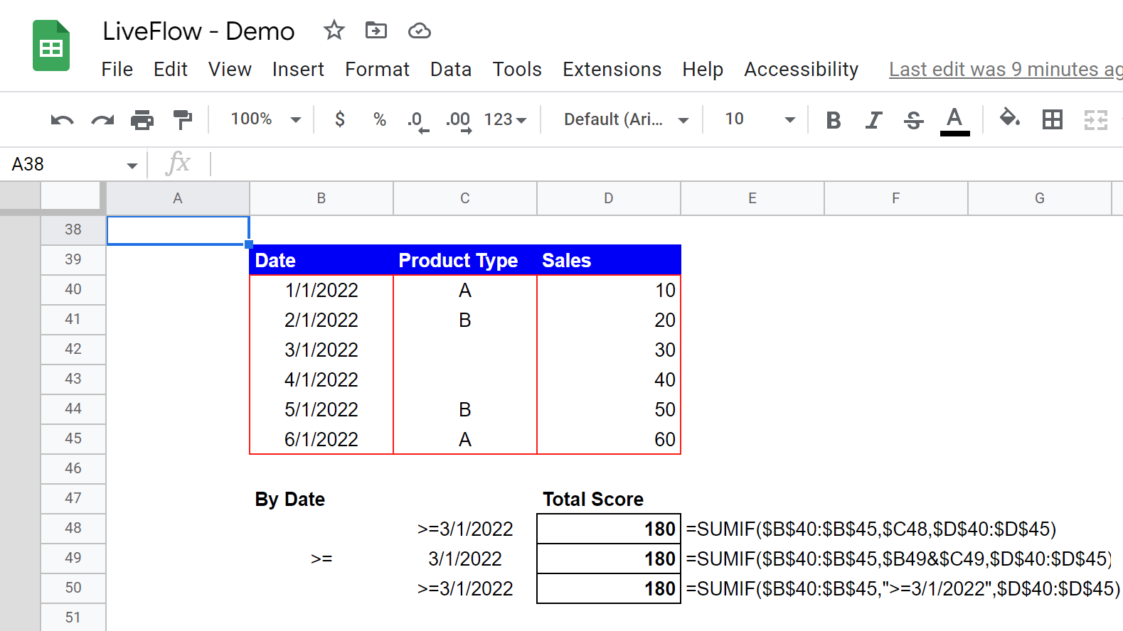
The difference between the two formulas is only in the logical operators: To include the threshold values in the sum, the greater than or equal to (>=) and less than or equal to (<=) operators are used.; To exclude the threshold numbers, use greater than (>) and less than (<).; For example, to sum the numbers in the range C2:C10 that are greater than 200 and less than 300, the formula is:
How to Use Google Sheets Sumif Multiple Criteria to Automate Your Spreadsheets Tech guide
Explanation of the SUMIF Formula in Google Sheets for This Example. In this example, the SUMIF formula Google Sheets checked each cell from A2 to A10 and looked for only those cells that contained the value "Packaging." For each cell that contains the word "Packaging," the SUMIF function selected its corresponding sales value in column B.It then added all the selected values and.

Google Sheets SUMIF Function Axtell Solutions
In this video, you will learn how to use Sumifs basics using Google Sheets. You also learn how to do sumifs using multiple with multiple criteria and columns.
SUMIF Multiple Criteria Google Sheets (Easiest Way in 2023)
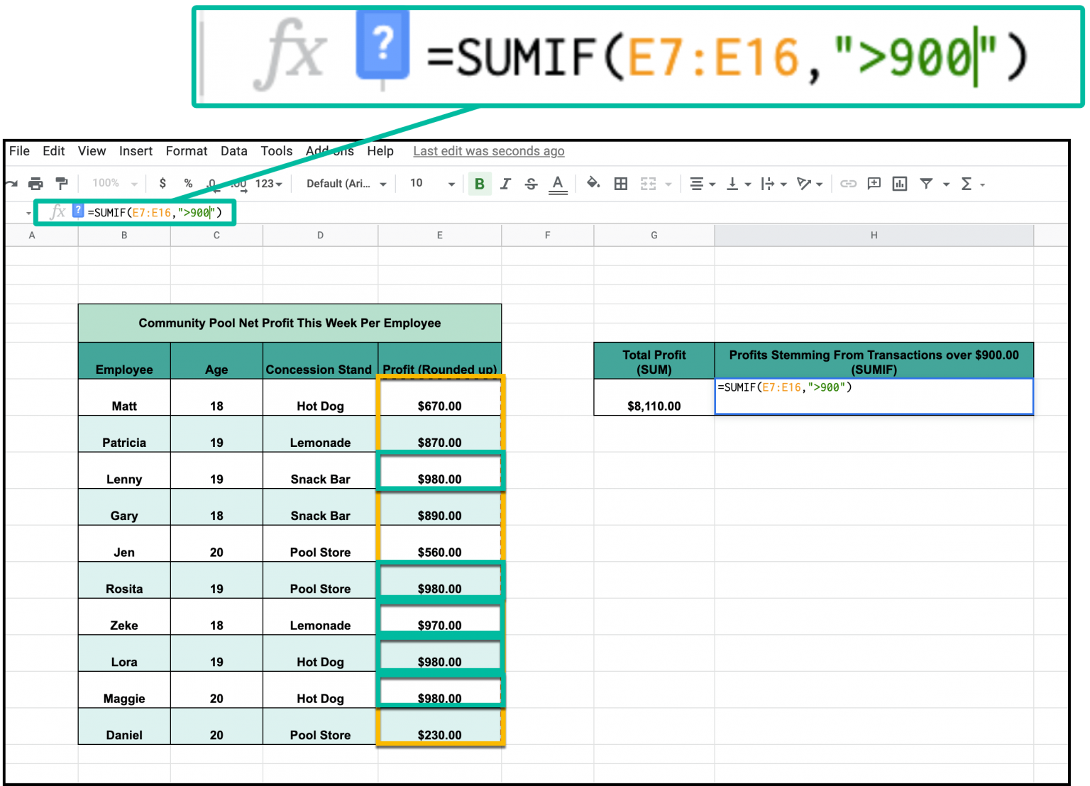
Use the SUMIF function in Google Sheets to add up specific cells of data. You can use the SUMIF function in Google Sheets to add up numbers across a range of cells if they meet the conditions. You might use this to summarize data in a category, such as adding up movie box office sales since 2015.
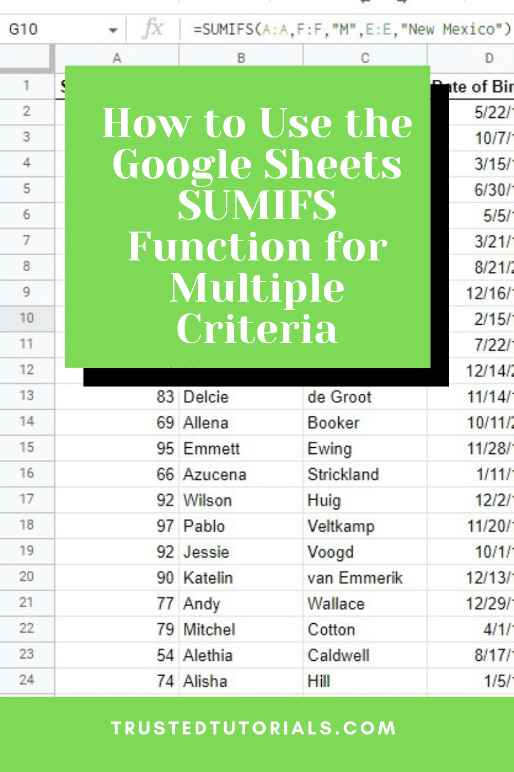
Google Sheets SUMIFS Function for Multiple Criteria
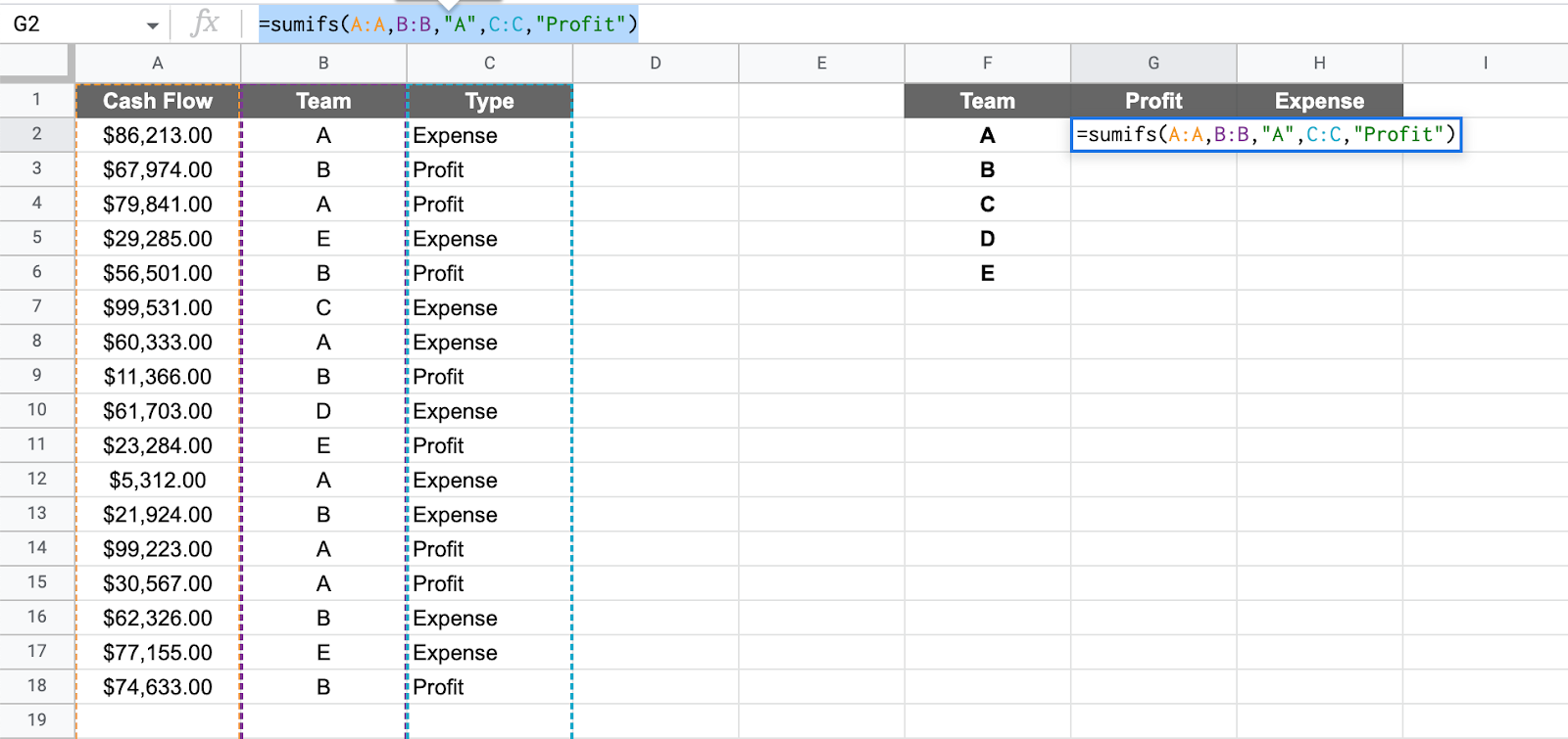
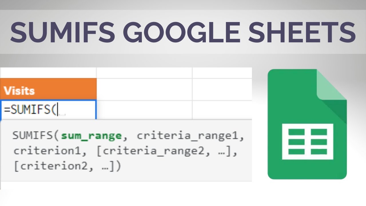
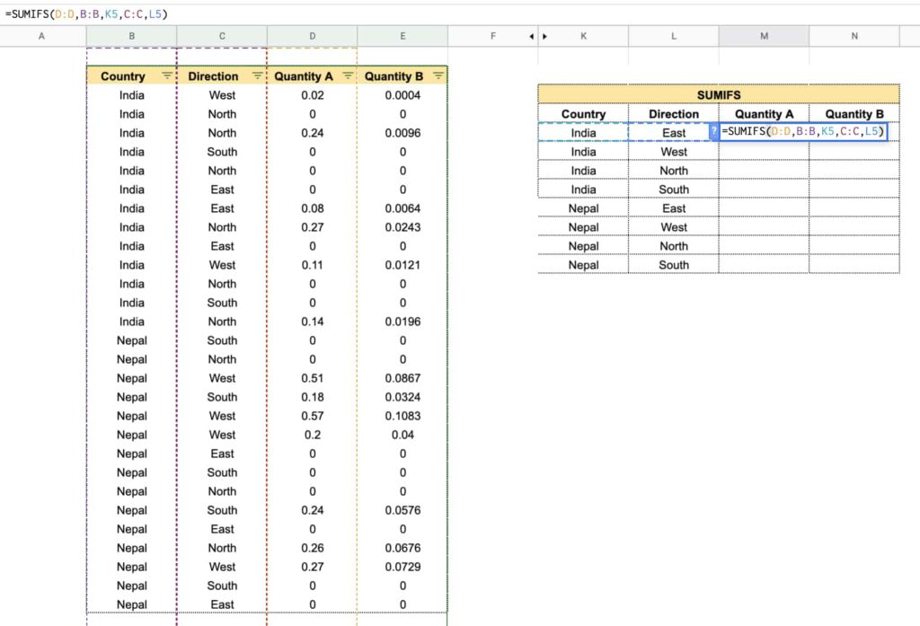
The SUMIFS () function in Google Sheets can be used to sum values that meet criteria in multiple columns. This function uses the following syntax: SUMIFS (sum_range, criteria_range1, criterion1, criteria_range2, criterion2,.) where: sum_range: The range of cells to sum. criteria_range1: The first range of cells to look at.
SUMIF Multiple Criteria Google Sheets (Easiest Way in 2023)
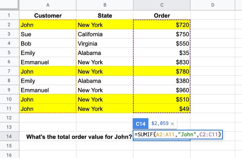
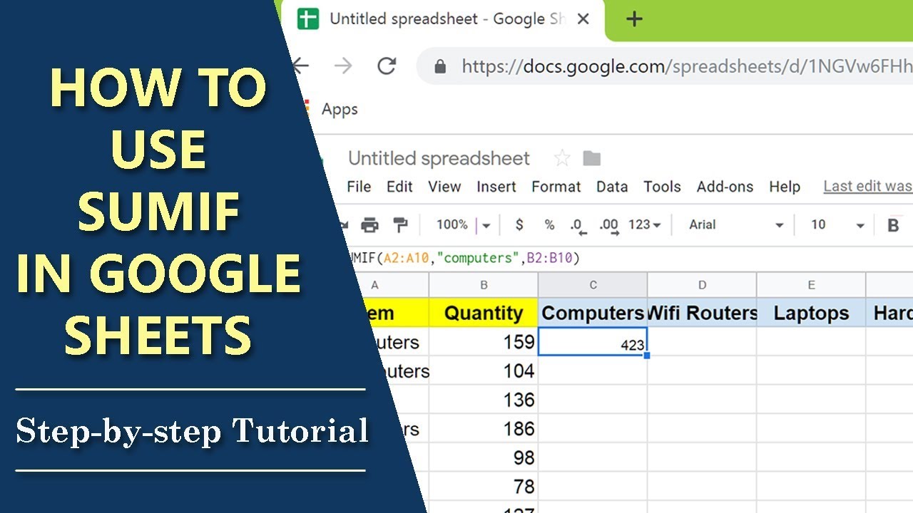
Use the SUMIF Function in Google Sheets The syntax for the function is SUMIF (cell_range, criteria, sum_range) where the first two arguments are required. You can use the sum_range argument for adding cells in a range other than the lookup range. Let's look at some examples. Related: How to Find Data in Google Sheets with VLOOKUP

How to Use SUMIF Contains in Google Sheets Statology
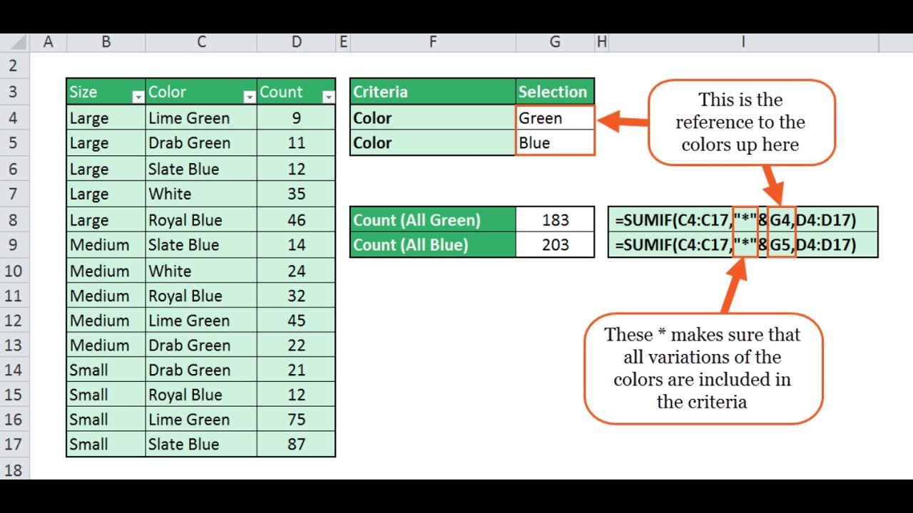
In this article we will show how to use SUMIF with multiple criteria in Google Sheets using the SUMIFS function. Simply follow the steps below: SUMIF Multiple Criteria Google Sheets Once you learn how to use the SUMIF function, it might be tempting to use it for multiple criteria.
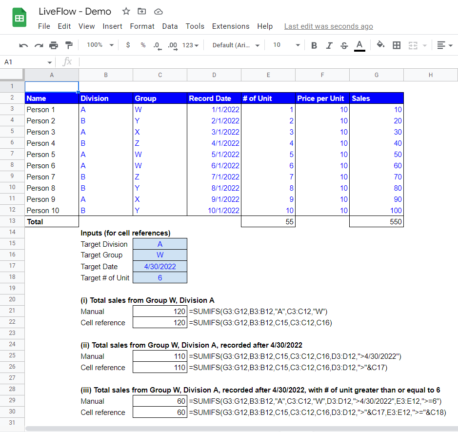
How to Use SUMIF Function in Google Sheets LiveFlow
Syntax SUMIF (criteria_column, criterion, sum_column) criteria_column - The data column which is tested against criterion. criterion - The pattern or test to apply to criteria_column..
How To Use Google Sheets SUMIF Function
The syntax and arguments for the SUMIF function in Google Sheets are as follows: SUMIF (range, criterion, [sum_range]) range: This is the range of cells that you want to evaluate against a specific criterion. It is a required argument and can be a row, a column, or a set of selected cells. criterion: This is the condition or rule that each cell.
How to use SUMIF in Google Sheets YouTube
To code a multiple criteria Sumif formula in Google Sheets, you should use the function ArrayFormula together with Sumif. Another requirement is the use of the & that joins multiple criteria and corresponding columns. Why don't you use the Sumifs instead? The reason Sumifs formula can't expand. In other words, it returns a single cell output.
How to use the SUMIF Function in Google Sheets
SUMIF: Returns a conditional sum across a range. SUMSQ: Returns the sum of the squares of a series of numbers and/or cells. SERIESSUM: Given parameters , , , and a, returns the power series sum a 1 x n + a 2 x (n+m) +. + a i x (n+ (i-1)m), where i is the number of entries in range `a`. QUOTIENT: Returns one number divided by another, without.
How to use the SUMIF function in Google Sheets to find a specific sum in your spreadsheet
November 8, 2023 • Zakhar Yung The most primitive way to total cells in Google Sheets is to add the cell references to the formula and put plus ( +) signs between them. For example: =B1+B2+B3+B4+B5 For longer ranges of cells, such as an entire column or row, this solution is not handy at all.
SUMIFS Google Sheets Multiple criteria on columns YouTube
The SUMIF function is Google Sheets is designed to sum numeric data based on one condition. Its syntax is as follows: SUMIF (range, criterion, [sum_range]) Where: Range (required) - the range of cells that should be evaluated by criterion. Criterion (required) - the condition to be met. Sum_range (optional) - the range in which to sum numbers.
Google Sheets SUMIF How to Use SUMIF Formula StepbyStep Tutorial YouTube
Its syntax is as follows: =SUMIF (range, criterion, [sum_range]) Where the variables mean the following attributes: range (required) is the range of cells that should be evaluated by the criterion. criterion (required) is the condition to be met. It can contain a number, a text, a date, a logical expression, a cell reference or any function.
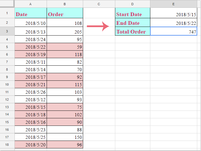
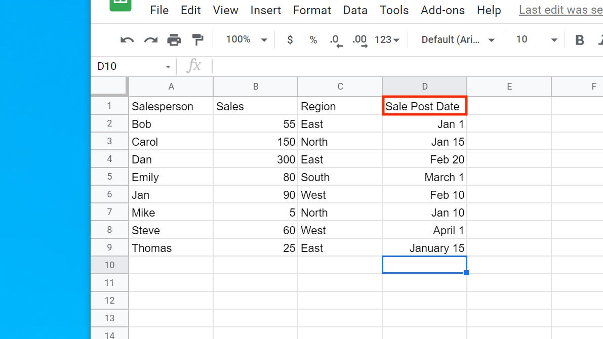
How to sumif cell values between two given dates in Google sheets?
The SUMIF function in Google Sheets is not suitable for this type of calculation, as it does not take two range parameters. The suggested function is SUMIFS. There are workarounds for this, such as combining the range and criteria.
Google Sheets SUMIFS and SUMIF with multiple criteria formula examples Tech guy ninja
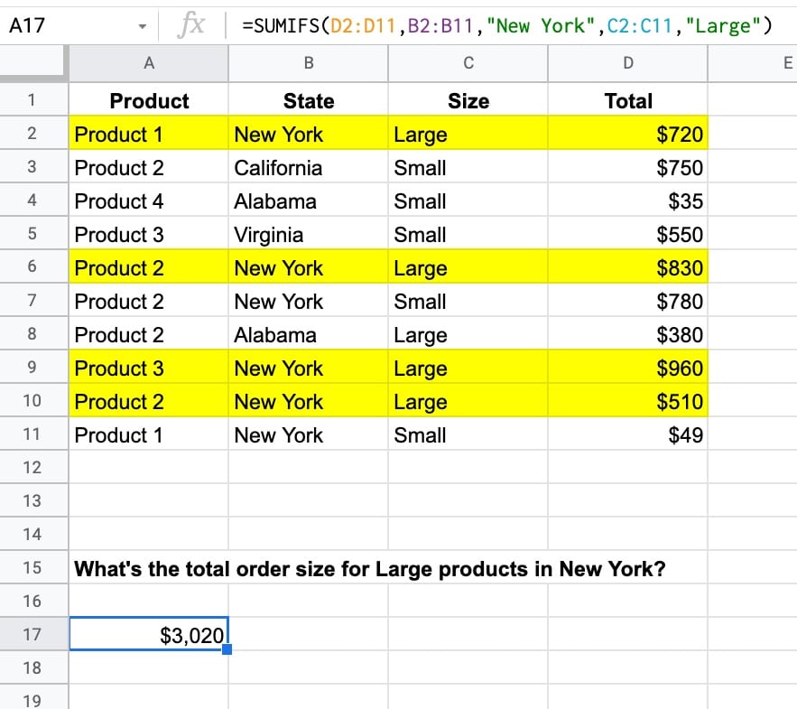
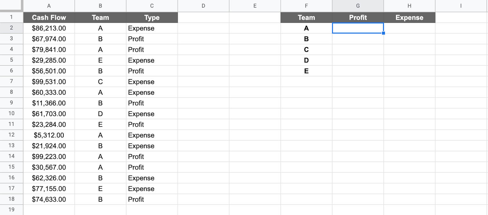
The SUMIFS function in Google Sheets enables you to sum values in your spreadsheet based on predefined conditions. Unlike the SUMIF function, which adds values to a sum based on a single condition, SUMIFS can enforce two or more conditions. The Google Sheets SUMIFS function only adds a value to a sum when all these conditions are met.